Understanding precision agriculture

THIS ARTICLE IS the third in a series intended to introduce and explain the concept of management zones, to provide a process to define, delineate, and characterize management zones, and to outline the kinds of data and computer tools needed to be successful. Previously, an overview of creating and characterizing management zones and the importance of multi-year yield data were discussed (go to www.gfo.ca/research/precisionag to read articles you may have missed).

As we continue to build toward understanding the spatial management component of precision agriculture, this article will explore the role of elevation/topography data for developing precision agriculture strategies associated with defining and using management zones.

UNDERSTANDING TOPOGRAPHY
Topography is often described by the pattern and magnitude of the slopes observed across a field.  Some common terms used to describe topography include level, nearly level, inclined, steep, hilly, rolling, gently undulating, and hummocky. For example, level is defined as a flat or very gently sloping one directional surface with a generally constant slope (<2%) not broken by knolls or depressions. Hummocky topography by contrast, is a very complex sequence of slopes (5% to 70%) extending from rounded depressions of various sizes to irregular knolls. Both hummocky and level topographies are commonly found in rural Ontario.

Topography is the dominant factor in controlling the flow and accumulation of water, organic matter, and other material in landscapes, which in turn affects the development and properties of soils. Topography influences the removal and deposition of soil materials by water, wind, and tillage practices. It impacts and affects soil salinity, pH, leaching, root zone development, mineral formation, and many other soil and site characteristics (adapted from MacMillan, 20031).

TECHNOLOGY
Collecting elevation data with as much accuracy and resolution as possible is very important and only has to be done once in a lifetime if done accurately. On the farm, a real time kinematic (RTK) global positioning system (GPS) is the only reliable and repeatable GPS source for this task.

An elevation data point consists of three numbers, an X (easting/ longitude) and Y (northing/latitude) coordinate and an elevation value, Z, in metres above sea level.

When using RTK-GPS to collect elevation data points, it is important to achieve suitable data quality. Ensure that your paths across the field (transects) are between five to 10 metres apart with the distance between data points within a pass one to three metres apart. In some cases, especially where the topography varies considerably, there is real value to making your passes narrower by collecting the data with an ATV or tractor mounted system (when the tractor is not pulling an implement).

During the elevation data collection process, the operator should ensure there is a consistent connection with the base station. Mobile base stations may be located in close proximity to the field (one to three kilometres away). For repeatable accuracy over time, the mobile base station location must be identified clearly so that it can be set up in the exact same location on each future use. This can be done by staking the location used in the first mapping session. Some choose to purchase and install a permanent base station at the farm. This is highly accurate; however, signals can degrade when fields are more than three to five kilometres from its location. Another popular choice for an RTK-GPS correction source for topography data is known as Virtual Reference Station (VRS). In order to use this option, you must be within the coverage area of the VRS network, have a GPS receiver that is capable of connecting to the VRS network, and a cellular data plan to provide the GPS receiver with an internet connection to the VRS network.

RTK-GPS elevation data should be reviewed for errors, such as missing data points due to a lost signal, to ensure that the data is accurate and consistent across the field.

USES OF ELEVATION DATA
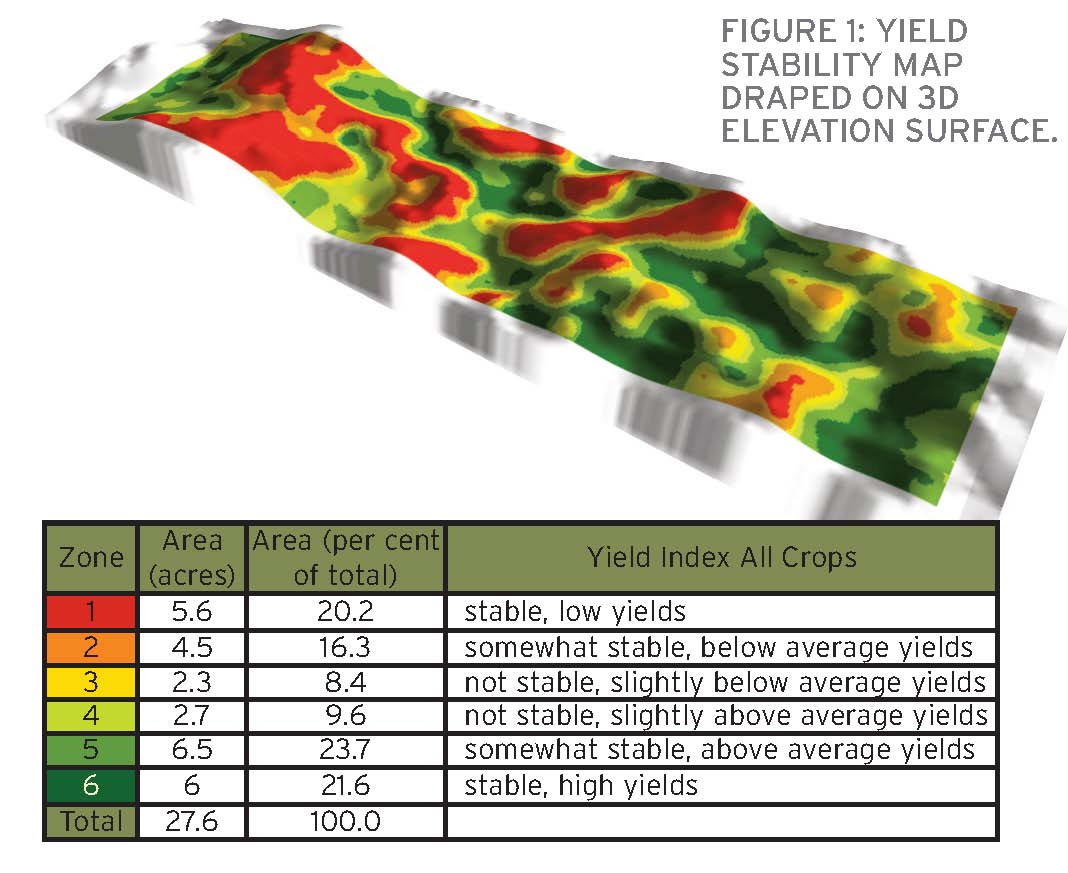
A 3D representation, known as a digital elevation model (DEM), of the topography of a field can be constructed from the data points collected by RTK-GPS. When additional data layers (ie. yield, CEC, soil chemistry, and NDVI) are combined with DEM you will create a clearer picture of field variability.

For example, Figure 1 shows a yield pattern stability map draped over the DEM. This shows that yields are strongly related to topography. Below average yield zones are associated with knolls, and high yielding areas are found in low areas or depressions.

TOPOGRAPHICAL TERRAIN LAYERS
A variety of terrain layers can be derived from a DEM that can be used to segment a field into zones. Where sufficient years of yield data do not exist, topographical zones can be substituted to develop management zones.

Terrain layers that are commonly used for making management zone maps, prescription maps, detailed soil type maps, or soil property maps include: per cent slope, aspect, topographic wetness index, and curvature, among others.

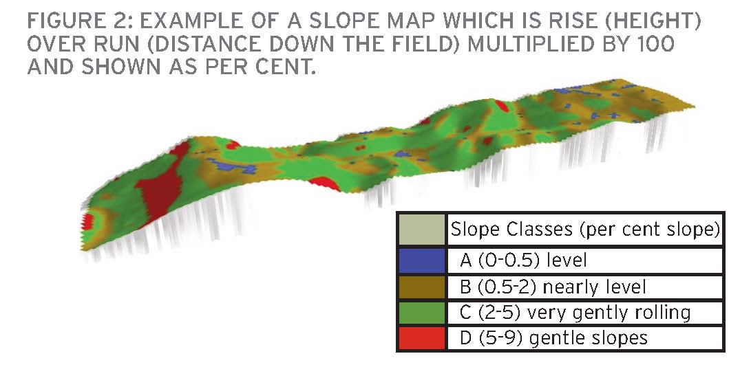
Slope is a measure of the steepness of a surface (Figure 2). It can be measured in degrees from horizontal (0-90), or per cent slope. The slope affects the rate of water movement downslope.

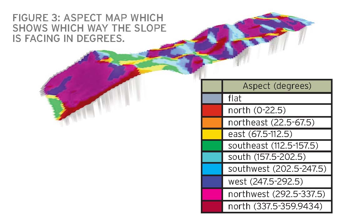
Aspect is the compass direction that a slope faces, usually measured in degrees from north (Figure 3) and defines the direction of water flow on a slope.

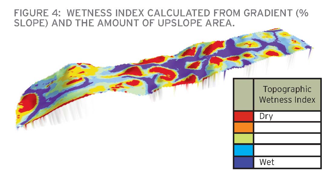
The wetness index (Figure 4) provides a measure of the relative likelihood of a point in the landscape being wetter or drier than normal, due to runoff from higher elevations.

Curvature is used to describe the shapes found on a slope.  Although there are several types of curvature that can be computed from a DEM, there are two primary curvatures which are of the greatest interest: downslope curvature, also known as profile, and across slope (planform) curvature. Downslope curvature affects the speed of water flow down a slope and therefore influences erosion and movement of soil and water. Across-slope curvature relates to the convergence (accumulation) or divergence (loss) of flow across a surface. Combining the downslope and across-slope curvatures helps to more accurately understand the movement of water and soil on slopes within a field.

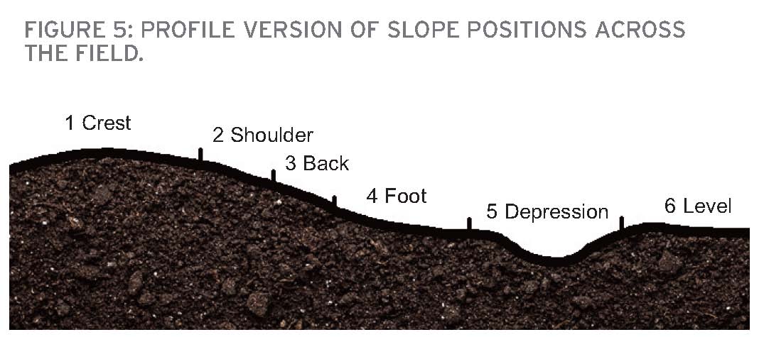
Relative slope position is a measure of the vertical height of a point in the landscape above a “stream” channel. This index is used to position a point in the field that occupies an upper slope, mid slope, or lower slope position.

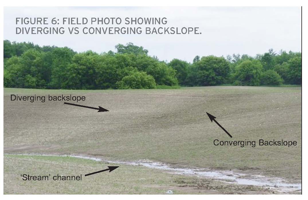
Slopes can be further subdivided into slope positions (Figure 5). A diverging and converging backslope combination is shown in Figure 6. The lighter colour of the diverging backslope is an indication of loss of soil and organic matter. The darker soil colour of the converging backslope is due to accumulation of organic matter. Converging backslopes are prone to gully formation under intense rainfall events.

RELATIONSHIP OF YIELD AND TOPOGRAPHY
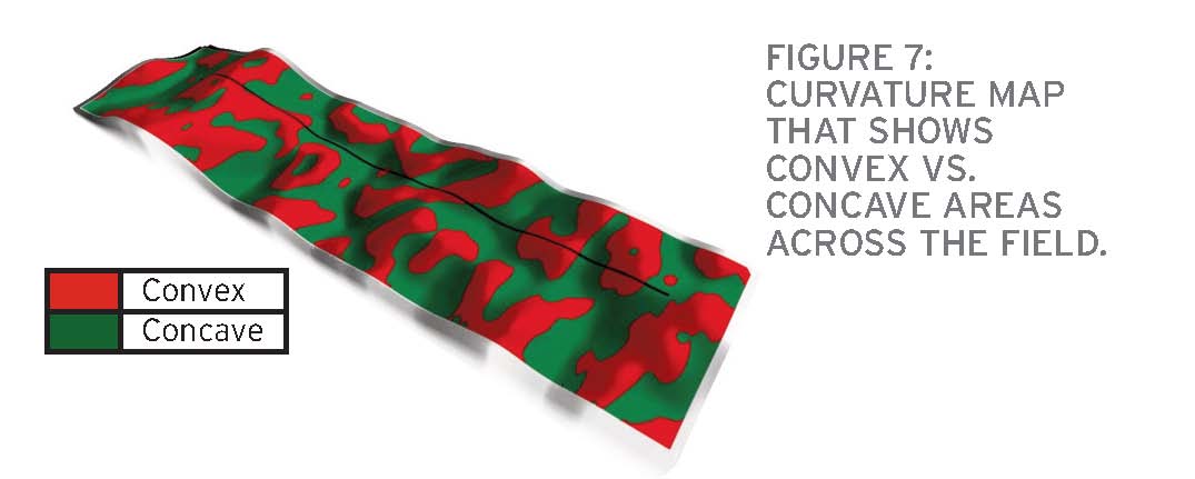
When comparing the yield pattern stability map to a convex and concave curvature map (Figure 7), you can see that yield and topography are very strongly correlated (compare Figure 1 and Figure 7).

The 3D yield pattern stability map (Figure 1) shows low yield areas where the convex areas (red) are shown on the curvature map (Figure 7). Note that high yields are associated with concave sections of the field, and below average yields are found on the convex areas of the field. One or more yield limiting factors are often found on the knolls. These include soil moisture deficits, excessive stoniness, low or high pH values, thin top soils with low organic matter levels, and poor soil structure.

Since we have established that there is a strong relationship between yield stability patterns and topography, it is reasonable to create management zones from elevation data that mimics the yield patterns. The curvature map can be used to create management zone maps. Figure 8 is an example of a curvature map with three zones: upper, mid, and lower slope positions.

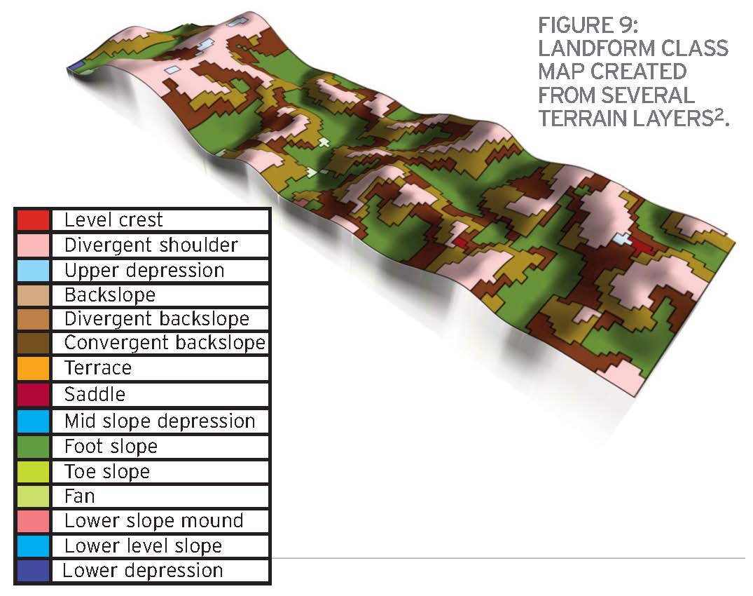
This technique of defining management zones in lieu of multi-year yield data has the greatest chance of success on fields with quite a bit of topography. This can be accomplished with a single topographical layer but a more detailed landscape segmentation, called a landform class map, can be created by using several topographical layers. Figure 9 was created using seven topographical layers including:  relative slope position, lowest relative point in a depression, absolute height above the lowest point in the field (metres), per cent slope, downslope curvature, across slope curvature, and wetness index.

Using a landform class map as a substitute to a multi-year yield map is possible in a precision agriculture strategy but the validity of this approach needs to be assessed carefully on a field-by-field basis. Landform class maps could be used in a variable rate fertilizer or population strategy that includes validation against conventional farm practices.

This article illustrates that elevation data and topographic modelling are very important in visualizing and developing reliable, repeatable/ stable management zones. If an Ontario grower does not have several years of yield data then it is logical to look at using good quality elevation data and terrain layers as a way to develop a site specific precision agriculture strategy for fields that have considerable topographic variability.

The next article in our series will explore soil information (physical and chemical) as we continue to build towards having all the possible layers that one might use to define stable and reliable management zones. •

1    MacMillan, R. A. 2003. LandMapR© Software Toolkit- C++ Version: Users manual. LandMapper. Environmental Solutions Inc., Edmonton, AB. 110 pp.
2    Surfer© and Saga-GIS software was used to compile the landform class map)